Creating an expected points (xP) calculator for Football matches
Expected points (xP), like expected goals (xG), attempts to put into context how likely certain events are to happen. For xG, this is the likelihood of a goal being scored from a certain shot. As for xP, this calculates the likelihood of each result (based on the shots in the match and their xG) and the number of points each team could expect on average to win given their xG performance.
Using xG to analyse how ‘fair’ a result was has become increasingly more common within the footballing world. By calculating xP you can more insight into a teams performance from game-to-game than just viewing their xG-difference. You can create an xP table (sometimes called a ‘justice table’) to see how many points each team could expect to have gained based on their accumulated xG in each game they have played.

Calculating xP in this basic model is not a complex task. You take all the shots within the game and simulate them to get the number of goals each team scored within this particular simulation of the game (which will then give you the result). After performing this over a significant number of simulations (whilst keeping track of all the results) you can calculate the proportion of times that team 1 wins, team 2 wins or the teams draw. From this, you can work out the xP by finding the number of points each team would achieve on average from these simulations.
I coded this in python, where I ask the user for inputs for xG values for each team. They can input until all the shot values are entered where a blank input will quit the loop and continue the code. If an input is entered, the program will check if it is valid. A valid input, in this case, is a number that is between 0 and 1. This is because xG is a probability of a shot resulting in a goal. If the input is valid, the xG value is added to a list for that team that contains each shots xG value. This process is repeated for the other team, ‘Team 2’.

After this, the user is prompted to input the number of simulations that they want the program to perform. The higher the number of simulations, the closer the program gets to the ‘true’ values. I found that 10,000 simulations gives a fairly accurate prediction calculation whilst keeping runtime to a minimum. This input obviously needs to be an integer so the program checks for this.

The step after this is to simulate the games. We do this n times (where n is the number inputted in the previous step) and during each simulation, each shot is simulated to see if it resulted in a goal. This is performed using the random module in python. For example, imagine simulating a shot with an xG of 0.2. A random number generated between 0 and 1 will give a number below 0.2 20% of the time and above 0.2 (or equal to due to how the random module works) 80% of the time. By checking this randomly generated number compared to the xG value for the shot we can see if the shot was predicted to be in. If the randomly generated number was less than the xG value then the shot was deemed to be scored. If it is higher then it is not scored. In this example, the shot with 0.2 xG will have a random number generate that is lowered than it 20% of the time, which accurately represents this shots’ xG.
Once all the shots have been simulated, the number of goals scored by each team can be compared and the obvious logic is used to check the result.

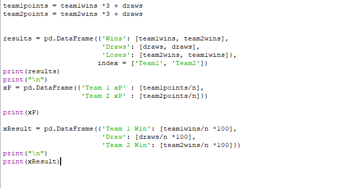
All that remains now is to present the data. We can work out the number of points each team achieved during the simulation by multiplying the number of wins they got by 3 and adding the number of draws. I decided to utilise the pandas module to create data frames to store the data in. This enables the data to be displayed easily within a table format.
I create 3 tables for each simulation. The first displays the number of wins, draws and losses that each team gets. The next shows the xP for each team, which is found by dividing the teams' total points by the number of games. The final table displays the probability of each result. This is calculated by dividing the number of times each result occurred by the total number of games and multiplying by 100. The code is below.
I will be showing an example of this program using data from the match on 16/01/21 between Leicester and Southampton which finished 2–0 to Leicester. The xG scoreline was approximately 2.1–0.4 in favour of Leicester (depending on the model you look at). I find that finding xG data for a team in total is easy but finding the xG value for each shot in the game is harder to find. I found that understat is the best resource for this information. According to their data, Leicester had 16 shots with Southampton having 8, with an xG scoreline of 2.12–0.38. We can enter each shots xG value into our program and simulate over a larger number of games (100,000) to the expected results for this game based on the shots.
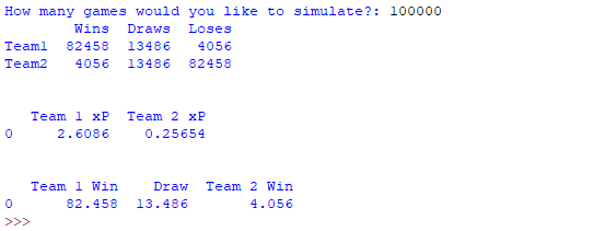
As we can see, given the shots in the match, Leicester (who are ‘Team 1’) had an xP of approximately 2.61 and expected to win the game 82.458% of the time. Southampton on the other hand (‘Team 2’) had an xP of about 0.26 and probability of winning of only 4.056%. Understat gives the xP values that they calculate themselves and give this as 2.61- 0.25 which is extremely close to the model's output. The slight variation might be due to a different model, a larger number of simulations or using xG values to more than 2 decimal places.
This program can also be used to check games that had ‘unexpected’ scorelines relative to the xG scorelines and see how unlikely they truly were. An example of a game that seems to have given a result that is contradictory to the xG scoreline is the match between Tottenham and Arsenal on 06/12/2020. The match finished 2–0 to Tottenham with an xG scoreline of 0.39-0.60. Despite how the game might have appeared to a spectator, this gives the impression that Arsenal had a slight edge over the course of the match. Simulating the game 100,000 times gives us the following results.
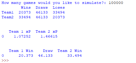
The results show that the most likely result was a draw, with Tottenham (Team 1) only expecting to win the game with these chances 20.373% of the time. This implies the possibility of a ‘lucky’ result despite how the game actually played out (which leads to further discussions about game states and xG accumulation for a team who are sitting on a lead). The xP scoreline of approximately 1.07–1.47 is close to understat’s who give a scoreline of 1.05–1.49.
Expected points give a purely objective look on a game to predict the outcome based only on the shots that occurred. The model does not look at any contextual information such as the game state. An example of this is a team that is pushing hard for a late equaliser. They might leave themselves more vulnerable to a counter which could give the team countering a seemingly inflated xG score. If the team breaks and accumulates a larger xG score whilst the other team are pushing this would not be representative of the game as a whole and only happened due to the state of the game. This is where weighted xG comes in and considers these scenarios.
Fundamentally, the amount of shots that occur in a football match is quite small so a large amount of variance is expected in this data which is why the ‘expected’ result ceases to happen a large proportion of the time.
